Polyhedral Compilation: How Compilers Turn Loops Into Geometry

A deep intuition-first dive into affine loops, dependence analysis, Pluto scheduling, tiling, and how modern compilers mathematically optimize code.

What is Polyhedral Compilation ?

The core of polyhedral compilation is basically a mathematical framework for analysing and transforming loops in programs. Before diving into the math, let us first understand what problem is this solving.

The Problem It Solves

Modern CPUs are fast but memory is slow. What I mean by that is that when a program runs nested loops like matrix multiplication, the pattern in which you access memory determines if your program is gonna run in 1 second or 10 seconds. The question is : “can a compiler automatically figure out the best loop structure for a given piece of hardware?” That’s exactly what polyhedral compilation does.

Before we dive in I think there are couple of concepts we should be aware about. So lets understand those first.

What is an “Affine Program”?

Now the first and foremost step is to understand an “Affine Program”. Polyhedral compilation works on a restricted but very common class of loops called the affine loops. These have :

1. Loop bounds that are linear functions of outer loop variables or constants (e.g., i = 0 to N, j = i to N)

2. Array accesses that are linear (affine) functions of loop variables (e.g., A[i+j], not A[i*j])

3. No data-dependent control flow inside the loop body

These are basically programs where everything behaves in a predictable, straight-line way (linear).

Example :

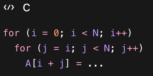
Here as you can see everything is linear :

1. i < N → simple

2. j = i to N → depends linearly on i

3. A[i + j] → linear

Everything is just addition, subtraction and constants.

Most scientific, ML, and image-processing kernels (matrix multiply, convolution, stencil computations) fall squarely into this class.

Now you might get a doubt that “why are we restricting to only linear/affine expressions?” The simple answer is that linear program form flat shapes (planes, boxes, cubes). Whereas non-linear bounds would give complex curved surfaces which we can’t evaluate easily.

Why Does This Matter

Computers (compilers) can easily understand and manipulate straight shapes, but not curved ones.

---

Affine case:

Like a grid or rectangle

You can:

• divide it into blocks (tiling)

• reorder it

• analyze it easily

---

Non-affine case:

Like a weird curved shape

You can’t:

• divide it cleanly

• reason about dependencies easily

• apply math optimizations safely

The reason we restrict to affine programs only is because they create simple, straight-line patterns that can be analyzed and optimized mathematically.

The Three Mathematical Objects

Now that we know what affine loops are, lets see their representation. Every affine loop nest gets represented as three things :

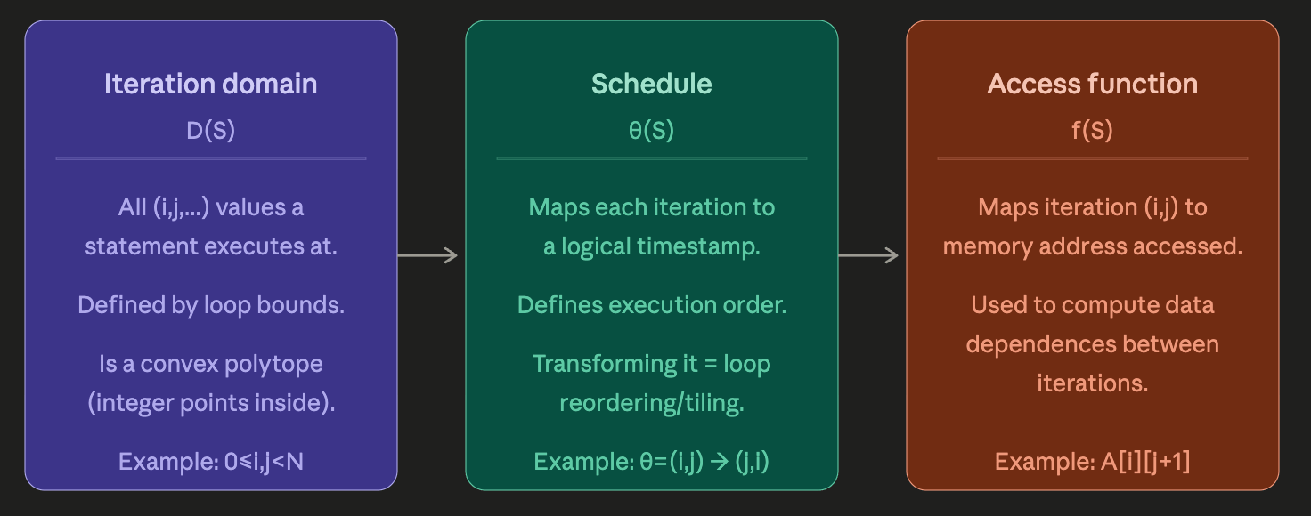
• Iteration Domain → WHERE computations happen

• Schedule → WHEN computations happen

• Access Function → WHAT memory each computation touches

Let Us Understand All Three Objects In Detail

Iteration domian

Let us take the following loop as an example

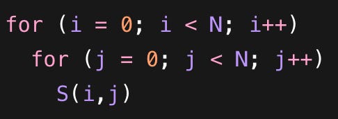
Iteration domain basically tells us all (i,j) values where the loops runs.

So : 0 ≤ i < N & 0 ≤ j < N

Think of each iteration as a point in the plane. So you get (0,0), (0,1), ……, (N-1,N-1). Which will be just a grid of points.

In short, iteration domain means all the points where computation happens.

Schedule

This basically tells us in what order should we execute these points.

The default schedule is

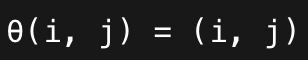
Which means sort by :

1. i

2. then j

Execution order :

which is a row-wise execution.

The transformation that happen like (tiling, interchange, etc.) are just changing of the schedule.

Access Function

Now we ask, when we are at (i,j), which memory location do we access ?

Access function tells us which memory location each iteration touches. The reason Iteration functions are important is because this is where dependencies come from.

The access function maps an iteration point to an array element.

A[i][j] is the function (i,j) → (i,j).

A[i][j+1] is (i,j) → (i, j+1).

Example:

(i, j) reads A[i][j-1]

Which was written by:

(i, j-1)

---

So dependency:

(i, j-1) → (i, j)

This is how the compiler knows:

1. what must come before what

2. what transformations are safe

Dependency Analysis

Now before transforming loops, the compiler must ensure it doesn’t break the required execution order between iterations. Basically it means if I reorder loops, the program should still produce the correct result.

That’s it, the entire topic revolves around this one thing.

The reason modern compiler reorder loops is to make programs run faster and they do this by :

• parallelizing loops

• tiling loops for cache efficiency

• interchanging loops

• fusing loops

• vectorizing loops

For example the compiler may transform:

for (i=0; i<N; i++)
  for (j=0; j<M; j++)

into:

for (j=0; j<M; j++)
  for (i=0; i<N; i++)

But before doing this the compiler has to make sure it doesn’t change the meaning of the program because some iterations depend on others.

When are Iterations Independent ?

We can understand this using a very simple example :

for (i = 0; i < 4; i++)
   A[i] = 10;

Here each iteration touches a completely different memory location. So no iterations affect each other and the loop can run in parallel. So because of this the compiler can reorder iterations safely.

When do Iterations Depend on Each Other ?

Lets take another example for this :

for (i = 1; i < 4; i++)
  A[i] = A[i-1] + 1;

This might look similar but is very different in terms of how memory is accessed. Lets understand this in more detail.

Iteration i = 1

A[1]=A[0]+1;

Touches:

• READ A[0]

• WRITE A[1]

Iteration i = 2

A[2]=A[1]+1;

Touches:

• READ A[1]

• WRITE A[2]

The important thing to notice here is :

1. At iteration i = 1, we write A[1]

2. At iteration i = 2, we read A[1]

So both the iterations touch the same memory location. And because of this it creates a relationship :

i = 2 depends on i = 1

because iteration 2 needs the value produced by iteration 1.

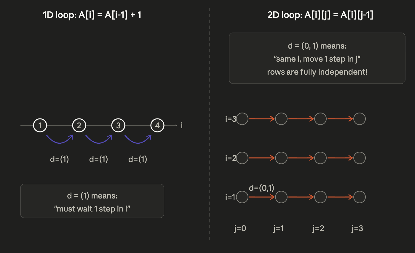
Dependence Vector

Now that we know that some iterations are dependent on each other, dependence vector tells us how far apart are these dependent iterations.

Lets take this example again :

for (i = 1; i < 5; i++)
    A[i] = A[i-1] + 1;

We already know that iteration i=2 depends on iteration i=1 because i=2 reads A[1] which was written by i=1.

When iteration q depends on iteration p (meaning p must run before q), the dependence vector is simply:

d = q - p

It’s the difference in coordinates between the two iterations. That’s it. For the loop above, p = 1 and q = 2, so:

d = 2 - 1 = (1)

The vector (1) means: “there is a dependence that jumps exactly 1 step forward in i.” For all pairs in this loop:

• i=2 depends on i=1 → d = (1)

• i=3 depends on i=2 → d = (1)

• i=4 depends on i=3 → d = (1)

Every dependence has the same distance. The dependence vector is uniform here.

Dependence Direction Vector

We know dependence vector tells us the exact numeric distance i.e +1 or +2 or (0, +1) etc.. but dependence direction vector tell us only the direction i.e forward ? , backward ? or same ?

Instead of numbers, it uses symbols :

1. “ < “ means Forward

2. “ > “ means Backward

3. “ = “ means same

Lets take a simple example to understand this clearly :

for (i = 0; i < N; i++)
  for (j = 1; j < M; j++)
    A[i][j] = A[i][j-1] + 1;

At iteration (i,j) it reads A[i][j-1] which was written by (i,j-1). So dependence is (i,j-1) → (i,j)

Dependence Vector (Consumer - Producer) gives us :

(i,j) — (i,j-1) = (0, +1)

Meaning there is :

1. No movement in i

2. forward movement in j

Why direction vector matter more

Exact distances may change after transformations, but the direction should remain the same for the loop transformation to be legal.

Let us take Legal Loop Interchange :

Example 1 :

Suppose : direction is (=,<)

After interchange is (<,=)

This is still in forward direction, so this is Legal.

Example 2 :

If After interchange it produces this : (>,=) then it basically means a backward dependence which is illegal. Because Consumer executes before Producer.

So in short the Dependence vector tells us “Exactly how far the data flows” and Direction vector tells us “Which way the data flows”. A loop transformation is legal if it preserves the producer-before-consumer ordering, which usually means the transformed dependence direction vectors remain lexicographically forward (not backward).

The Omega Test and Fourier–Motzkin Elimination

So far we have understood dependency analysis conceptually:

• Two iterations depend on each other if they access the same memory location

• At least one access is a write

• The compiler represents accesses mathematically

• Then it checks whether valid iteration pairs exist

But now comes the important question : “How does the compiler actually solve these equations?”

This is where the “geometry” of polyhedral compilation comes into play. Underneath all the high-level compiler transformations is a math proof engine that answers questions like : “Do these constraints have a valid integer solution?”

Lets understand the whole pipeline :

1. Lets start up with loop example

for (i = 1; i < 5; i++)
    A[i] = A[i - 1] + 1;

We already know that Iteration 2 depends on Iteration 1 and that there is a dependence here.

1. What the Compiler Whats to know

The compiler asks “can two different iterations access the same array location?”. To reason this mathematically, it creates two copies of the loop variable :

• i₁ → first iteration

• i₂ → second iteration

Note : The compiler still doesn’t know that there is a dependence.

For dependence : They must access the same location, so compiler writes : i1 = i2 - 1

This equation basically means A value written by one iteration is read by another.

1. Why loop bounds matter

The compiler also knows :

for (i = 1; i < 5; i++)

So :

1 ≤ i1 ≤ 5
1 ≤ i2 ≤ 5

Now the question that compiler asks is do integer values exist satisfying all these equations.

1. Solve it manually

We have :

i₁ = i₂ - 1
1 ≤ i₁ < 5
1 ≤ i₂ < 5

If i2 = 2 then i1 = 1, which is valid. So dependency Exists.

The Entire Compiler Problem is Basically This

It repeatedly asks “Can I find valid integer values?”

If yes : Dependency Exists

If no : No Dependency

Fourier-Motzkin Elimination

This is basically a way of solving those equations by removing variables one-by-one until problem becomes simpler.

Suppose we have:

x + y ≤ 10
x ≥ 2

Rewrite first equation:

x ≤ 10 - y

Now:

2 ≤ x ≤ 10 - y

For this to be possible:

2 ≤ 10 - y

So:

y ≤ 8

Now the problem Fourier-Motzkin faces that it works over REAL numbers, but loops use intergers. This difference matters a lot.

Example :

2x = 1

Over real numbers:

x = 0.5

Valid answer, but loop iterations cannot be:

i = 0.5

Iterations must be integers.

Omega Test Intuition

To solve our previous problem faced by using Fourier-Motzkin, this test is basically a smarter interger-aware elimination algorithm. It extends Fourier-Motzkin while carefully handling integer rules.

Example

Suppose compiler gets:

2i₁ = 2i₂ + 1

Basically means:

even = odd

Which is impossible. The Omega Test detects this quickly.

The Reason this matters is because after this the compiler know if there is any dependence or not. So that it safely parallelize or reorder loops.

Okay till now we know that the compiler builds an iteration domain, detects dependencies and checks if the transformations are legal or not. But the important part that we have to understand is detecting whether a transformation is legal is different from finding the best one.

There are infinitely many valid loop orderings for a given program. The compiler has to figure out which one to pick. That is basically the Scheduling problem.

Scheduling Problem

As I mentioned earlier, a schedule is just a function that assigns a timestamp to every iteration point.

The default schedule for

for i: for j: is θ(i,j) = (i, j)

meaning sort first by “i”, then by “j”

Now imagine if you are allowed to change that function. You can try :

• θ(i,j) = (j, i) → loop interchange

• θ(i,j) = (i/B, j/B, i, j) → tiling

• θ(i,j) = (i+j, j) → skewing

All of these schedules are different but each one visits the same set of points just in different order. This compiler is basically searching through this huge space of possibilities and asking : which one runs faster on this hardware?

Now a valid schedule must satisfy two things simultaneously :

1. Legality : Every dependency has to be respected. If iteration “p” must run before iteration “q”, then the schedule must assign “p” a timestamp that comes before “q”. In short the schedule must keep all dependences pointing “Forward”.

2. Optimality : Among all the legal schedules, pick the one that minimizes execution time. On a modern CPU this mostly means: minimize how often you fetch data from RAM, and maximize how much work you do with data while it’s still in cache. On a multi-core machine it also means: maximize the number of iterations that can run in parallel.

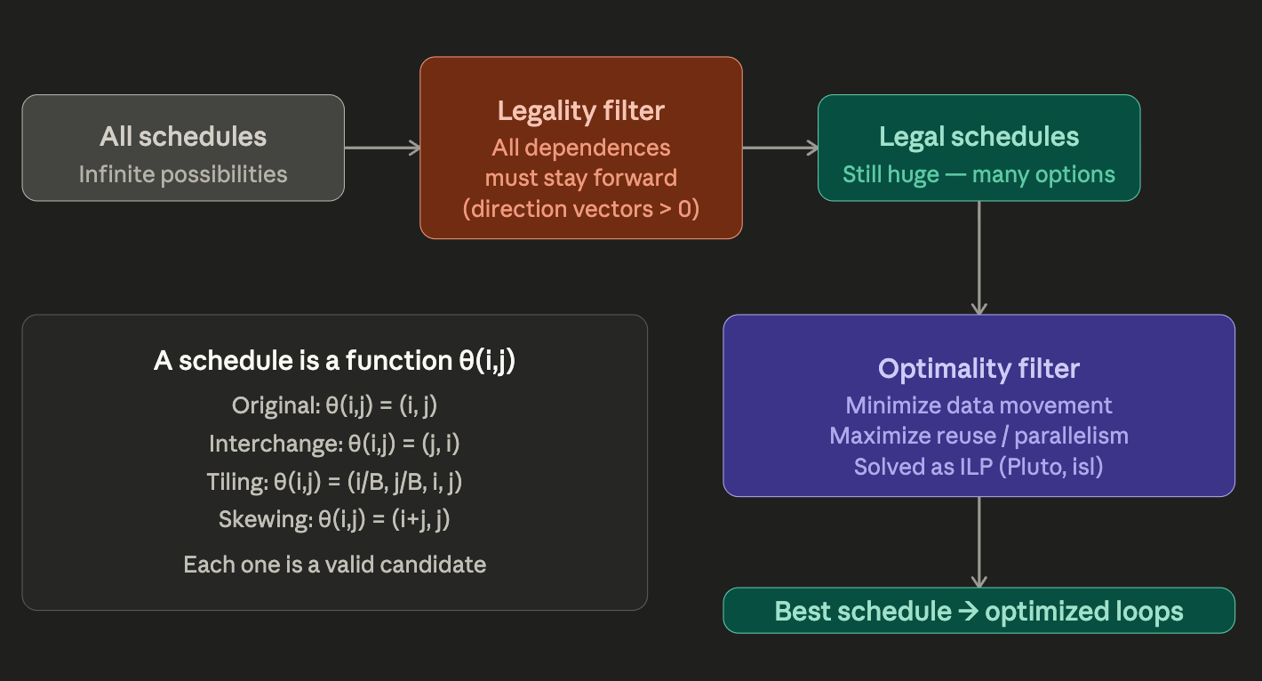
Now the compiler cannot go through all of these options because its not just large - its infinite. So we need to find a better and more optimal way to do it, which is exactly what Pluto provides.

The Pluto Algorithm

Pluto’s central idea is clever and straight forward. Instead of saying “’let me try all the different loop transformations and see which one is fastest” it says : “let me directly search for a schedule that maximizes data reuse, subject to legality constraints - and let the loop transformations fall out as a consequence.”

What Pluto is actually searching for

Pluto is looking for a schedule of the form θ(i,j) = c₁·i + c₂·j + c₀ a linear function of the loop variables. The unknowns are the coefficients c₁, c₂, c₀.

Finding the right coefficients indirectly means finding the right schedule.

For example:

• If c₁=1, c₂=0 → sort by i first → original order

• If c₁=0, c₂=1 → sort by j first → interchange

• If c₁=1, c₂=1 → sort by i+j → skewing

The transformation comes from these coefficients. Pluto doesn’t have a list of “try interchange, try tiling or try skewing”. It just solves for these coefficients and whatever is the solution, will be the transformation.

Lets try to understand a little back story to actually why we are using this Pluto Algorithm.

As I mentioned in the beginning of this blog, today’s CPUs are fast but memory is slow. What I actually mean by that is, whenever a program needs to run, it needs to fetch data. Now there are couple places where it can fetch the data from, it could either be RAM or cache.

Whenever a program needs data from RAM, it first tries to see if that data is already present in the cache.

• If the data is already there → then data is retrieved very fast (cache hit)

• If not → it has to go all the way to RAM → which is slow (cache miss)

So the biggest goal in loop optimization is:

“Use data again before it gets kicked out of the cache.”

This is what Pluto tries to optimize.

Let us understand using an example what I mean by “Use data again before it gets kicked out of the cache”

Example 1 : Consider this simple loop

for (i = 0; i < 3; i++) {
    for (j = 0; j < 3; j++) {
        use(A[i]);
    }
}

For i = 0, notice that

use(A[0])
use(A[0])
use(A[0])

The same value A[0] is reused many times immediately.

That is good for cache because once A[0] is loaded, it stays in cache while we keep using it for different iterations as well. Because of this it reduces the time fetching the data.

Example 2 :

for (j = 0; j < 3; j++) {
    for (i = 0; i < 3; i++) {
        use(A[i]);
    }
}

Now the accesses become:

A[0], A[1], A[2],
A[0], A[1], A[2],
A[0], A[1], A[2]

Here as we can see between two uses of A[0], many other values were accessed. Maybe cache already evicted A[0] so if we tried to access A[0] again we would have to go the RAM. That is worse locality.

What Pluto wants :

Pluto basically asks “Can I reorder iterations so reused data is accessed closer together in time?”

Because :

• close together in time = likely still in cache

• far apart in time = probably evicted

So Pluto tries to make reused values happen as soon as possible.

The Cost Function (the actual optimization target) :

The cost function basically means “what number are we trying to minimize of maximize?”

For Pluto it is : Cost = total dependence distance

Smaller cost means:

• producer and consumer iterations execute closer together

• reused data stays in cache

• fewer cache misses

• all of which leads to faster program

So Pluto searches for loop schedules that make this number as small as possible.

How the Compiler Actually Solves It

Now that we understand why Pluto wants better schedules, let’s try to understand how it actually computes them mathematically using ISL (Integer Set Library).

Think of Pluto as an optimization strategy and ISL as the mathematical engine underneath all of this.

When Pluto decides “I want a schedule that minimizes reuse distance.” Then at that point ISL is the thing that actually manipulates the equations, solves the constraints, and computes the schedule.

Let us tie all of this together with an example :

1. Represent Loops mathematically

for (i = 0; i < N; i++)
    for (j = 0; j < N; j++)
        S(i,j);

Now as we know Pluto converts this loop into an iteration space and each iteration becomes a point (i,j). So the entire loop becomes a 2D grid of points.

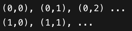
Lets take N = 3 :

(0,0) (0,1) (0,2)
(1,0) (1,1) (1,2)
(2,0) (2,1) (2,2)

ISL represents this as a polyhedron :

0 ≤ i ≤ N, 0 ≤ j < N

This is the basically the mathematical representation of the loop.

2. Dependencies Become Constraints

Now suppose iteration (i,j) produces a value used by (i, j + 1). That means (i,j) has to be executed before (i,j+1). Otherwise the program will become invalid, this is Pluto encodes as the legality constraint.

3. Pluto Introduces An Unknown Schedule

As we discussed earlier that Pluto doesn’t try to find all the legal loop transformation, instead it solves a linear schedule instead.

Now Pluto assumes an unknown linear schedule:

θ(i,j) = c1i + c2j + c0

The coefficients :

c₁, c₂, c₀

are unknown. Finding these coefficients means finding the execution order.

4. Converting Correctness Into Equations

Now we already know that the Producer must be executed before Consumer.

So Pluto writes :

θ(i , j+1) − θ(i , j) ≥ 1

Now substitute the schedule equation. After substitution we get :

(c1i + c2(j+1) + c0) − (c1i + c2j + c0) ≥ 1

Everything cancels except :

c2 ≥ 1

This is really important because the compiler just transformed program correctness into a linear inequality. ISL is actually really good at solving systems of inequalities like this.

5. Locality Becomes The Optimization Objective

At this point, Pluto has ensured that the schedule is correct, but that alone is not enough. There are many schedules which may satisfy the legality constraints. Now Pluto asks “Among all legal schedules, which one gives the best cache locality?”

This becomes the actual optimization objective.

Consider the slightly modified loop :

for (i = 0; i < N; i++)
    for (j = 0; j < N; j++)
        use(A[i]);

Here you can notice the accessed value only depends on i and not j.

That means :

(i=0,j=0) → A[0]
(i=0,j=1) → A[0]
(i=0,j=2) → A[0]

The same value is reused as j changes.

So reuse happens when : j changes while i stays fixed.

Because of this Pluto wants iterations differing only in “j”, to execute close together in time, because nearby accesses are likely to stay in cache.

Now consider the schedule agian :

θ(i , j) = c1i + c2j

The coefficient c2 controls how quickly the time changes as “j” changes. If c2 is very large, reused accesses become far apart in schedule time.

For example:

θ(i , j) = i+ 100j

gives:

Even though all these iterations reuse A[0], they execute very far apart in time. That increase the chances that A[0] gets evicted from cache before we get to reuse it.

So Pluto prefers smaller coefficients for dimensions where reuse occurs frequently. This intuition become the cost function (This is a simplified intuition for understanding locality optimization, not Pluto’s exact ILP objective) :

Cost = c1 + c2

Pluto now basically asks ISL to minimize the cost while still satisfying all legality constraints.

6. ISL Solves The Integer Linear Program (ILP)

At this point, Pluto has transformed the scheduling problem into pure mathematics.

It now has:

Constraints (correctness)

c2 ≥ 1

Objective (locality)

min⁡(c1 + c2)

This is a standard Integer Linear Program (ILP) and ISL solves this system mathematically and returns the best legal coefficients.

7. The schedule becomes a loop transformation

Suppose ISL returns :

c1 = 0

c2 = 1

Then the schedule becomes : θ(i , j) = j

This means sort the iterations primarily by j. Which corresponds to loop interchange.

For a different loop with a diagonal dependence, ISL might return c₁=1, c₂=1 giving:

θ(i , j) = i + j

then execution proceeds diagonally, which corresponds to loop skewing.

The important thing to know here is that Pluto never explicitly says :

“Perform interchange.”

“Perform skewing.”

“Perform tiling.”

It only tries to find the schedule coefficients that minimize reuse distance while preserving correctness.

Now Pluto has found the best loop order, but that alone is also not enough for large matrices. Even the best ordering still cause cache misses. So to solve this problem let us deep dive into Tiling.

What Problem Does Tiling Solve

Let us take an example of naive matmul and see why it destroys ours cache

for (i = 0; i < N; i++)
    for (j = 0; j < N; j++)
        for (k = 0; k < N; k++)
            C[i][j] += A[i][k] * B[k][j];

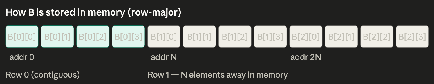
To understand the cache problem we need to know how arrays are stored in memory. They are stored in a row-major order. A 2D array A[row][col] is stored as one long line in memory. First all row 0, then all of row 1, and so on.

The important to understand is, the problem is NOT the multiplication itself, the problem is HOW memory is accessed.

Now now know that the actual memory layout is like this :

[B00 B01 B02 B03 B10 B11 B12 B13 B20 B21 B22 B23]

Suppose we access :

B[0][0]
B[0][1]
B[0][2]
B[0][3]

These are adjacent in memory and CPU cache loves this. The reason behind this is that cache loads memory in chunks called cache lines. Usually 64 bytes at once.

So when CPU loads : B[0][0] it automatically also fetches nearby values for free which are :

B[0][1]
B[0][2]
B[0][3]

This is called Spatial Locality where nearby memory gets reused, which is very efficient.

Now Lets Understand Why Columns Are Terrible

Lets say we access :

B[0][1]
B[1][1]
B[2][1]

Notice one thing here, that we are down a column. But remember our memory layout :

[B00 B01 B02 B03 B10 B11 B12 B13 B20 B21 B22 B23]

If we were look carefully we can find that

B[0][1] -> position 1
B[1][1] -> position 5
B[2][1] -> position 9

these are FAR apart in memory.

Now the reason this is a huge problem is because lets say we have a matrix size :

N = 1024 and each float occupies 4 bytes. Then : B[0][1] to B[1][1] is

1024 x 4 = 4096 bytes apart

But cache line size is only 64 bytes, so that means every access jumps FAR outside the current cache line. So every access needs a new RAM fetch which is going to be extremely slow and inefficient.

Now coming back to our original example of matrix multiplication :

for (i = 0; i < N; i++)
    for (j = 0; j < N; j++)
        for (k = 0; k < N; k++)
            C[i][j] += A[i][k] * B[k][j];

If notice carefully we have B[k][j] inside the innermost loop for(k). So here we are gonna access :

B[0][j]
B[1][j]
B[2][j]

that means walking down a column which we now know is cache-unfriendly.

Now Pluto’s loop interchange definitely helps, it may discover :

for(k)
    for(i)
        for(j)

Now for fixed K :

B[k][0]
B[k][1]
B[k][2]

These are being accessed sequentially, which means walking across rows instead of columns. Which is a HUGE improvement.

But even with perfect order : A, B, and C are still HUGE. Entire matrices cannot fit in cache. So eventually cache eviction still happens. We need to still reload data repeatedly. That is where Tiling comes into play.

The Gap That Tiling Fills

Tiling says “Don’t work on the whole matrix at once.” Instead work on tiny block that fit in cache. For example instead of processing 1024 x 1024 matrix process a 64 x 64 block at a time.

What the tiled loop looks like

The naive loop:

for (i = 0; i < N; i++)
  for (j = 0; j < N; j++)
    for (k = 0; k < N; k++)
      C[i][j] += A[i][k] * B[k][j];

The tiled loop with tile size B:

for (ii = 0; ii < N; ii += B)       // step through row-tiles
  for (jj = 0; jj < N; jj += B)     // step through col-tiles
    for (kk = 0; kk < N; kk += B)   // step through depth-tiles
      for (i = ii; i < ii+B; i++)   // work inside tile
        for (j = jj; j < jj+B; j++)
          for (k = kk; k < kk+B; k++)
            C[i][j] += A[i][k] * B[k][j];

The outer three loops (ii, jj, kk) move between tiles. The inner three loops (i, j, k) work inside one tile. The computation is identical, same multiplications, same additions, same result. But the memory access pattern is completely different.

Lets try to understand this by taking a small example :

1. Take a tiny matrix

Suppose : N = 4 , so matrices are 4x4. We’ll use tile size B = 2. So now the matrix gets divided into 2x2 blocks.

+----+----+
| T1 | T2 |
+----+----+
| T3 | T4 |
+----+----+

Each tile is a small square.

2. What We Do In Normal Multiplication

To compute C[0][0] we load :

A[0][0] A[0][1] A[0][2] A[0][3]

and

B[0][0] B[1][0] B[2][0] B[3][0]

Now later to compute for C[0][1] we AGAIN need many of the same A values. But the cache may have already evicted them. So we reload them which is an inefficiency.

3. What Tiling Does

Instead of computing just C[0][0] we compute :

C[0][0] C[0][1]
C[1][0] C[1][1]

All together. That 2x2 square is one tile.

4. Now Visualize The Reuse

To compute the output tile :

+---------+
| C00 C01 |
| C10 C11 |
+---------+

we load one small tile from A and one from B.

A tile :

A00 A01
A10 A11

B tile :

B00 B01
B10 B11

Once A00 is loaded into cache it gets reused for BOTH C00 and C01. Similarly B00 gets reused for BOTH C00 and C10.

Tiling is one of those concepts that becomes instantly obvious the moment you see it animated, if the memory access pattern isn’t clicking yet, searching for “cache tiling visualization” or “loop blocking animation” on YouTube will make it snap into place in seconds.

As for where tiling comes from in the compiler, it doesn’t get added as a separate step after Pluto. When Pluto is allowed to search over schedules that have a tile-index dimension and an intra-tile dimension for the same loop variable, the ILP it solves naturally lands on a tiled solution. The reason is straightforward: tiling is precisely what minimizes reuse distance when the full matrix doesn’t fit in cache. Pluto doesn’t know the word “tiling” is, it just finds the schedule with the smallest cost, and that schedule, when written out as loop code, is a tiled loop. The math basically forces it there.

Scanning The Polyhedron

Now the question this topic answers is after Pluto runs, the compiler has a transformed polyhedron, a mathematical object described as a system of inequalities.

You can think of these inequalities as describing a geometric region containing all valid loop iterations.

The inequalities can be something like :

0 ≤ ii < N, step B
0 ≤ jj < N, step B  
ii ≤ i < ii+B
jj ≤ j < jj+B
i < N
j < N

This is obviously not code and CPU cannot execute a system of inequalities. Someone has to look at this math object and write out the corresponding for loops with correct bounds. That process of turning a polyhedron back into loop code, is called scanning the polyhedron. That job is done by CLooG or ISL code generator.

How do they work ?

Now the question is:

“How does ISL/CLooG look at inequalities and actually generate nested for loops?”

The answer is simple :

They repeatedly ask: “For this dimension, what are the valid integer values?” That’s literally the entire algorithm.

Lets start with the simplest inequalities

Suppose ISL receives : 0 ≤ i < 4

This describes valid values of : i , So the compiler asks “What values can i take ?”

And the answer is : 0, 1, 2, 3

So code generator emits : for(i = 0; i < 4; i++)

That’s it.

Now Comes Tiling

Suppose the inequalities are :

0 ≤ ii < N

ii ≤ i < ii + B

i < N

Now compiler must generate loops for this particular inequality.

So compiler asks : “What values can ii take?”

Answer : 0 ≤ ii ≤ N with step size B.

So it emits :

for(ii = 0; ii < N; ii += B)

Now the compiler asks : “For this ii, what values can i take?” Compiler sees TWO upper bounds :

Constraint 1 : i < ii + B (tile Boundary)

Constraint 2 : i < N (matrix boundary)

Now to actually satisfy BOTH inequalities, we have to find the actual upper bound. And the answer to that is basically smaller of the two.

Which becomes : i < min(ii + B, N) and

The Lower bound comes from : ii ≤ i

So the generated loop becomes :

for(i = ii; i < min(ii+B, N); i++)

The reason why this min() function is important because the tile wants to continue until ii + B, but the matrix itself ends at N. Most tiles fit perfectly, but the last tile may partially fall outside the matrix.

So the compiler chooses whichever boundary comes first. That is how min() appears, the compiler sees two competing upper-bound constraints and takes the smaller one.

So CLooG/ISL are basically geometric interpreters, they take a look at a geometric region and ask : “What are the legal integer coordinates?” and then they systematically turn those coordinates into nested for loops by :

• picking one dimension

• finding its lower bound

• finding its upper bound

• emitting a loop

• moving inward recursively

This is the complete pipeline, from source code to optimized loops. The compiler builds the iteration domain, finds dependences, computes the best schedule via Pluto, and finally scans the resulting polyhedron to emit runnable code. In the next post we'll see where all of this lives in modern compilers: MLIR.

Conclusion

Polyhedral compilation looks intimidating at first because of all the math, inequalities, schedules, and optimization problems. But underneath all of it, the core idea is surprisingly simple:

A loop nest can be viewed as a geometric space of computations.

Once the compiler converts loops into mathematical objects, transformations that normally feel complicated like loop interchange, skewing, fusion, parallelization, or tiling become mathematical operations on that space.

The compiler is no longer “guessing” optimizations. It is proving which transformations are legal and then searching for schedules that improve locality and parallelism.

That is what makes the polyhedral model so powerful.

Modern systems like Pluto, ISL, and MLIR use these ideas to optimize scientific computing, machine learning kernels, stencil computations, and high-performance code generation. Even though the theory can become very deep, the entire pipeline fundamentally revolves around one question:

“How can we reorder computations without changing the meaning of the program, while making the hardware happier?”

And surprisingly, the answer turns out to be geometry.

I wrote this blog as part of my own journey learning polyhedral compilation and compiler optimizations. My goal here was not to give a fully rigorous research-level treatment, but to build an intuition-first understanding of how the entire pipeline fits together.

If you notice any mistakes, oversimplifications, or inaccuracies, please feel free to point them out. I’d genuinely appreciate corrections and deeper insights from people more experienced in this space.